#install.packages('librarian')
librarian::shelf(tidyverse, dataRetrieval, rnaturalearth)Code
This page houses a curated set of code examples designed to support students as they develop their own analytical frameworks. Rather than prescribing a single workflow, these examples introduce a range of R packages, functions, and approaches that students may, or may not be, accustomed to using in their own work. The goal is to expose students to different ways of working with data and to help them identify tools that are most appropriate for their research questions.
Students are encouraged to explore the code, modify it for their own purposes, and combine ideas across examples as their analyses. Code examples are grouped by theme (e.g., data retrieval, modeling, visualization).
Data Retrieval
Gathering hydrology data
Below we showcase code that can be used to gather data from stream gauges maintained by the United States Geological Survey (USGS) using the dataRetrieval package. While some of you may be aware of (or even familiar with) the package, there are some relatively new (as of 11/2025) features outlined by USGS here.
Housekeeping
Load necessary packages
if you do not have librarian installed, you will need to install it first
librarian() is nice because it automatically installs, updates, and attaches packages
First, we will use the readNWISdata() in the dataRetrieval package to pull all stream flow (CFS, i.e., parameter code 00060) data for the state of Ohio - the default is daily average (i.e., stat code **00003* as seen in rename()). Check out the link to peruse all the parameter codes and their associated information
site_hydro <- readNWISdata(stateCd = 'OH',
parameterCd = '00060',
startDate = '2023-12-01',
endDate = '2023-12-31') |>
janitor::clean_names() |>
rename(flow_cfs = x_00060_00003,
date = date_time) |>
mutate(year = year(date),
month = month(date),
day = day(date)) |>
select(date, year, month, day, site_no, flow_cfs)GET:https://waterservices.usgs.gov/nwis/dv/?format=waterml%2C1.1&stateCd=OH¶meterCd=00060&startDT=2023-12-01&endDT=2023-12-31I generally despise capital letters in column names, so I usually clean them up using the clean_names() function in the janitor package. I also frequently use the glimpse() function to make sure my code is running as planned.
glimpse(site_hydro)Rows: 6,973
Columns: 6
$ date <dttm> 2023-12-01, 2023-12-02, 2023-12-03, 2023-12-04, 2023-12-05, …
$ year <dbl> 2023, 2023, 2023, 2023, 2023, 2023, 2023, 2023, 2023, 2023, 2…
$ month <dbl> 12, 12, 12, 12, 12, 12, 12, 12, 12, 12, 12, 12, 12, 12, 12, 1…
$ day <int> 1, 2, 3, 4, 5, 6, 7, 8, 9, 10, 11, 12, 13, 14, 15, 16, 17, 18…
$ site_no <chr> "03090500", "03090500", "03090500", "03090500", "03090500", "…
$ flow_cfs <dbl> 37.1, 36.1, 35.7, 35.4, 35.1, 33.5, 33.3, 44.7, 49.6, 199.0, …Next, we can pull out the distinct() sites to look up further metadata using the readNWISsite() function for each site_no
sites <- site_hydro |>
distinct(site_no)
site_info <- readNWISsite(siteNumbers = sites$site_no) |>
select(site_no, station_nm, dec_lat_va, dec_long_va) |>
rename(lat = dec_lat_va,
lon = dec_long_va,
river = station_nm) |>
janitor::clean_names()GET:https://waterservices.usgs.gov/nwis/site/?siteOutput=Expanded&format=rdb&site=03090500,03091500,03092090,03092460,03093000,03094000,03094704,03095500,03098600,03098700,03099500,03109500,03110000,03111500,03111548,03113990,03114306,03115400,03115644,03115712,03115786,03115917,03116000,03116077,03116196,03117000,03117500,03118000,03118500,03120500,03121500,03124500,03125900,03126000,03126910,03127000,03128500,03129000,03129197,03136500,03139000,03140000,03140500,03141500,03141870,03142000,03144000,03144500,03144816,03145000,03145173,03145483,03145534,03146000,03146402,03146500,03149500,03150000,03150500,03156400,03157000,03157500,03159500,03159540,03202000,03205470,03216070,03217424,03217500,03219500,03219781,03220000,03221000,03221646,03223425,03225500,03226800,03227107,03227500,03228300,03228500,03228689,03228750,03228805,03229500,03229610,03229796,03230310,03230427,03230450,03230500,03230700,03230800,03231500,03232000,03232300,03232500,03234000,03234300,03234500,03237020,03237280,03237500,03238495,03240000,03241500,03244936,03245500,03246500,03247500,03255349,03255420,03259000,03260706,03261500,03261950,03262000,03262500,03262700,03263000,03264000,03265000,03266000,03266560,03267000,03267900,03269500,03270000,03270500,03271000,03271300,03271500,03271620,03272000,03272100,03272700,03274000,03322485,04177000,04177266,04178000,04180988,04181049,04183500,04183979,04184500,04185000,04185318,04185440,04185935,04186500,04187100,04188100,04188252,04188324,04188337,04188400,04188433,04188496,04189000,04189131,04189174,04189260,04190000,04191058,04191444,04191500,04192500,04192574,04192599,04193500,04193999,04195500,04195820,04196000,04196500,04196800,04197100,04197137,04197152,04197170,04198000,04199000,04199155,04199500,04200500,04201400,04201409,04201423,04201484,04201495,04201500,04201526,04202000,04203900,04206000,04206413,04206416,04206425,04206448,04207200,04208000,04208347,04208460,042085017,04208502,04208684,04208700,04208923,04209000,04212100,04213000,394653084072100,402913084285400,402958084363300,410014081362600,410051081594500,410121081330300,410433081312500,411607084241200,411610084240800,412141081412100,412325081415500,412453081395500,412624081450700glimpse(site_info)Rows: 225
Columns: 4
$ site_no <chr> "03090500", "03091500", "03092090", "03092460", "03093000", "0…
$ river <chr> "Mahoning River bl Berlin Dam nr Berlin Center OH", "Mahoning …
$ lat <dbl> 41.04839, 41.13145, 41.16145, 41.15700, 41.26117, 41.23922, 41…
$ lon <dbl> -81.00120, -80.97120, -81.19705, -81.07176, -80.95426, -80.880…Lastly, we can pull the site hydrology and spatial information together using a left_join() function.
hydro <- site_hydro |>
left_join(site_info) |>
mutate(year = year(date),
month = month(date),
day = day(date)) |>
select(date, year, month, day, river, site_no, flow_cfs, lat, lon)Joining with `by = join_by(site_no)`For those not familiar, left_join() is one of many join functions. I have attached a pretty robust introduction to these here. However, to be frank.. I rarely use anything other than left_join() (though see anti_join()), though I am certain there are reason to. Another good article here.
glimpse(hydro)Rows: 6,973
Columns: 9
$ date <dttm> 2023-12-01, 2023-12-02, 2023-12-03, 2023-12-04, 2023-12-05, …
$ year <dbl> 2023, 2023, 2023, 2023, 2023, 2023, 2023, 2023, 2023, 2023, 2…
$ month <dbl> 12, 12, 12, 12, 12, 12, 12, 12, 12, 12, 12, 12, 12, 12, 12, 1…
$ day <int> 1, 2, 3, 4, 5, 6, 7, 8, 9, 10, 11, 12, 13, 14, 15, 16, 17, 18…
$ river <chr> "Mahoning River bl Berlin Dam nr Berlin Center OH", "Mahoning…
$ site_no <chr> "03090500", "03090500", "03090500", "03090500", "03090500", "…
$ flow_cfs <dbl> 37.1, 36.1, 35.7, 35.4, 35.1, 33.5, 33.3, 44.7, 49.6, 199.0, …
$ lat <dbl> 41.04839, 41.04839, 41.04839, 41.04839, 41.04839, 41.04839, 4…
$ lon <dbl> -81.0012, -81.0012, -81.0012, -81.0012, -81.0012, -81.0012, -…For a look at the spatial distribution of gauges, lets do a quick plot
hydro |>
group_by(site_no, lat, lon) |>
summarize(flow_m = mean(flow_cfs, na.rm = TRUE),
.groups = 'drop') |>
ggplot(aes(x = lon, y = lat, color = log1p(flow_m))) +
borders("state", regions = "ohio",
color = "black", linewidth = 0.6, fill = NA) +
geom_point(size = 3, alpha = 0.9) +
scale_color_viridis_c(option = "magma") +
theme_classic() +
labs(x = "Longitude", y = "Latitude",
color = 'log(Mean CFS)')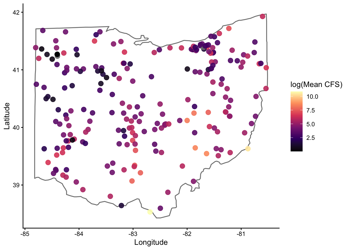
For those unfamiliar, the borders() function is very coarse, but good for a quick look like this
Next, we will use the readNWISdv() in the dataRetrieval package to pull stream flow (CFS) data for a list of sites, as opposed to the entire state as done above
First, we will create a list of sites with their site numbers. I have chose to use the tribble() function here. For those unfamiliar with tribble(), I have added some background information about tables, tibbles, and tribbles (oh my) here. When dealing with a lot of different sites it will be best to enter data into an excel document and read it in, however.
site_hydro <- tribble(
~river, ~siteNumber,
"Scioto-Columbus", "03227500",
"Maumuee-Defiance", "04192500",
"Little Muskingum-Bloomfield", "03115400",
"Little Miami-Milford", "03245500",
"Hocking-Athens", "03159500",
"Olentangy-Deleware", "03225500",
)Now that we have our sites, it is time to pull the flow data (parameter code 00060) for all sites using the map() function in the purrr package. For those unaware, the map() function will change your left if you let it. Ditch the for loops and join us in the tidyverse. See video here for full explanation of the map() function, as well as map_dbl() and map_dfr() :)
hydro <- site_hydro |>
mutate(
data = map(
siteNumber,
~readNWISdv(
siteNumbers = .x,
parameterCd = '00060',
startDate = '2023-12-01',
endDate = '2023-12-31'
)
)
) |>
dplyr::select(river, siteNumber, data) |>
unnest(data) |>
rename(flow_cfs = X_00060_00003,
date = Date) |>
dplyr::select(river, flow_cfs, date) |>
mutate(year = year(date),
month = month(date),
day = day(date)) |>
dplyr::select(date, year, month, day,
river,
flow_cfs)GET:https://waterservices.usgs.gov/nwis/dv/?site=03227500&format=waterml%2C1.1&ParameterCd=00060&StatCd=00003&startDT=2023-12-01&endDT=2023-12-31GET:https://waterservices.usgs.gov/nwis/dv/?site=04192500&format=waterml%2C1.1&ParameterCd=00060&StatCd=00003&startDT=2023-12-01&endDT=2023-12-31GET:https://waterservices.usgs.gov/nwis/dv/?site=03115400&format=waterml%2C1.1&ParameterCd=00060&StatCd=00003&startDT=2023-12-01&endDT=2023-12-31GET:https://waterservices.usgs.gov/nwis/dv/?site=03245500&format=waterml%2C1.1&ParameterCd=00060&StatCd=00003&startDT=2023-12-01&endDT=2023-12-31GET:https://waterservices.usgs.gov/nwis/dv/?site=03159500&format=waterml%2C1.1&ParameterCd=00060&StatCd=00003&startDT=2023-12-01&endDT=2023-12-31GET:https://waterservices.usgs.gov/nwis/dv/?site=03225500&format=waterml%2C1.1&ParameterCd=00060&StatCd=00003&startDT=2023-12-01&endDT=2023-12-31Take a quick glimpse to make sure all went as planned
glimpse(hydro)Rows: 186
Columns: 6
$ date <date> 2023-12-01, 2023-12-02, 2023-12-03, 2023-12-04, 2023-12-05, …
$ year <dbl> 2023, 2023, 2023, 2023, 2023, 2023, 2023, 2023, 2023, 2023, 2…
$ month <dbl> 12, 12, 12, 12, 12, 12, 12, 12, 12, 12, 12, 12, 12, 12, 12, 1…
$ day <int> 1, 2, 3, 4, 5, 6, 7, 8, 9, 10, 11, 12, 13, 14, 15, 16, 17, 18…
$ river <chr> "Scioto-Columbus", "Scioto-Columbus", "Scioto-Columbus", "Sci…
$ flow_cfs <dbl> 382, 327, 238, 229, 255, 279, 237, 227, 351, 530, 372, 783, 7…Next (and just for fun), I wanted to highlight how to use the map2() function, also maintained within the purrr package. Where map() iterates a function over a single vector or list, map2() iterates a function over (you guessed it) two vectors or lists.
I have set everything up according to our first example below. However, in this example I want to pull flow and temperature data from these sites so I need to specify that in terms of parameter codes (i.e., site_params). I also need to make sure that flow and temperature data is retrieved for all sites (where available). To create a data frame with all unique combinations of site and parameter code, I used the crossing() function.
site_hydro <- tribble(
~river, ~siteNumber,
"Scioto-Columbus", "03227500",
"Maumuee-Defiance", "04192500",
"Little Muskingum-Bloomfield", "03115400",
"Little Miami-Milford", "03245500",
"Hocking-Athens", "03159500",
"Olentangy-Deleware", "03225500"
)
site_params <- tribble(
~parameterCd, ~var,
'00060', 'FlowCFS',
'00010', 'WaterTempC'
)
cross <- crossing(site_hydro, site_params)hydro_and_temp <- cross |>
mutate(data = map2(
siteNumber,
parameterCd,
~readNWISdv(
siteNumbers = .x,
parameterCd = .y,
startDate = "2023-12-01",
endDate = "2023-12-31"
)
)) |>
dplyr::select(river, siteNumber, parameterCd, var, data) |>
unnest(data) |>
rename(flow_cfs = X_00060_00003,
temp_c = X_00010_00003,
date = Date) |>
mutate(year = year(date),
month = month(date),
day = day(date)) |>
dplyr::select(date, year, month, day, river, flow_cfs, temp_c) |>
pivot_longer(flow_cfs:temp_c, names_to = 'metric', values_to = 'value') |>
na.omit() |>
arrange(metric)GET:https://waterservices.usgs.gov/nwis/dv/?site=03159500&format=waterml%2C1.1&ParameterCd=00010&StatCd=00003&startDT=2023-12-01&endDT=2023-12-31GET:https://waterservices.usgs.gov/nwis/dv/?site=03159500&format=waterml%2C1.1&ParameterCd=00060&StatCd=00003&startDT=2023-12-01&endDT=2023-12-31GET:https://waterservices.usgs.gov/nwis/dv/?site=03245500&format=waterml%2C1.1&ParameterCd=00010&StatCd=00003&startDT=2023-12-01&endDT=2023-12-31GET:https://waterservices.usgs.gov/nwis/dv/?site=03245500&format=waterml%2C1.1&ParameterCd=00060&StatCd=00003&startDT=2023-12-01&endDT=2023-12-31GET:https://waterservices.usgs.gov/nwis/dv/?site=03115400&format=waterml%2C1.1&ParameterCd=00010&StatCd=00003&startDT=2023-12-01&endDT=2023-12-31GET:https://waterservices.usgs.gov/nwis/dv/?site=03115400&format=waterml%2C1.1&ParameterCd=00060&StatCd=00003&startDT=2023-12-01&endDT=2023-12-31GET:https://waterservices.usgs.gov/nwis/dv/?site=04192500&format=waterml%2C1.1&ParameterCd=00010&StatCd=00003&startDT=2023-12-01&endDT=2023-12-31GET:https://waterservices.usgs.gov/nwis/dv/?site=04192500&format=waterml%2C1.1&ParameterCd=00060&StatCd=00003&startDT=2023-12-01&endDT=2023-12-31GET:https://waterservices.usgs.gov/nwis/dv/?site=03225500&format=waterml%2C1.1&ParameterCd=00010&StatCd=00003&startDT=2023-12-01&endDT=2023-12-31GET:https://waterservices.usgs.gov/nwis/dv/?site=03225500&format=waterml%2C1.1&ParameterCd=00060&StatCd=00003&startDT=2023-12-01&endDT=2023-12-31GET:https://waterservices.usgs.gov/nwis/dv/?site=03227500&format=waterml%2C1.1&ParameterCd=00010&StatCd=00003&startDT=2023-12-01&endDT=2023-12-31GET:https://waterservices.usgs.gov/nwis/dv/?site=03227500&format=waterml%2C1.1&ParameterCd=00060&StatCd=00003&startDT=2023-12-01&endDT=2023-12-31Gathering land use data
CAP presented the StreamCatTools package for pulling land use data. While I have not had time to put together a formal demonstration of its utility, I have linked the packages GitHub site here
Data Wrangling
Linking trait data
Below we showcase code that can be used to generate a ‘species’ list and link it to an existing trait dataset
Housekeeping
Load necessary packages
if you do not have librarian installed, you will need to install it first
#install.packages('librarian')
librarian::shelf(tidyverse, skimr)Similar to above, I am using the tribble() and crossing() functions to generate simulate some data. I am coupling these functions with the rlnorm() function to create an example count dataset of fishes commonly encountered in the state of Ohio
species <- tibble::tribble(
~common_name, ~family, ~genus, ~species,
"Largemouth Bass", "Centrarchidae", "Micropterus", "salmoides",
"Smallmouth Bass", "Centrarchidae", "Micropterus", "dolomieu",
"Bluegill", "Centrarchidae", "Lepomis", "macrochirus",
"Channel Catfish", "Ictaluridae", "Ictalurus", "punctatus",
"Flathead Catfish", "Ictaluridae", "Pylodictis", "olivaris",
"Common Carp", "Cyprinidae", "Cyprinus", "carpio",
"Gizzard Shad", "Clupeidae", "Dorosoma", "cepedianum",
"Emerald Shiner", "Cyprinidae", "Notropis", "atherinoides",
"Creek Chub", "Cyprinidae", "Semotilus", "atromaculatus",
"Logperch", "Percidae", "Percina", "caprodes"
)
sites <- tribble(
~river,
"Scioto-Columbus",
"Maumuee-Defiance",
"Little Muskingum-Bloomfield",
"Little Miami-Milford",
"Hocking-Athens",
"Olentangy-Deleware",
)
years <- tibble(year = 2000:2025)
dat <- crossing(species, sites, years) |>
select(year, river, common_name, family, genus, species) |>
mutate(count = round(rlnorm(n(), meanlog = 1, sdlog = 1)))glimpse(dat)Rows: 1,560
Columns: 7
$ year <int> 2000, 2001, 2002, 2003, 2004, 2005, 2006, 2007, 2008, 2009…
$ river <chr> "Hocking-Athens", "Hocking-Athens", "Hocking-Athens", "Hoc…
$ common_name <chr> "Bluegill", "Bluegill", "Bluegill", "Bluegill", "Bluegill"…
$ family <chr> "Centrarchidae", "Centrarchidae", "Centrarchidae", "Centra…
$ genus <chr> "Lepomis", "Lepomis", "Lepomis", "Lepomis", "Lepomis", "Le…
$ species <chr> "macrochirus", "macrochirus", "macrochirus", "macrochirus"…
$ count <dbl> 17, 5, 2, 4, 2, 1, 1, 1, 4, 5, 2, 3, 1, 7, 1, 5, 1, 1, 4, …I am going to take a similar approach to generate an example trait dataset
traits <- tibble::tribble(
~species,
~max_length_mm, ~age_maturity_yr, ~longevity_yr, ~egg_size_mm,
~mean_clutch_size, ~parental_care,
~larval_growth_mm_mo, ~yoy_growth_mm_yr, ~adult_growth_mm_yr,
~spawn_season_d,
"Largemouth Bass", 600, 3.5, 14, 1.8, 120000, 3, 15, 120, 40, 90,
"Smallmouth Bass", 550, 4.0, 12, 2.0, 90000, 3, 14, 110, 38, 80,
"Spotted Bass", 500, 3.0, 11, 1.7, 85000, 3, 14, 105, 36, 85,
"Bluegill", 300, 2.0, 8, 1.2, 45000, 2, 18, 95, 32, 110,
"Redear Sunfish", 350, 2.5, 9, 1.4, 52000, 2, 17, 100, 33, 105,
"Green Sunfish", 280, 1.8, 7, 1.1, 40000, 2, 19, 90, 30, 115,
"Channel Catfish", 800, 5.0, 18, 5.5, 18000, 5, 10, 85, 30, 60,
"Flathead Catfish", 1100, 6.0, 22, 6.2, 9000, 6, 9, 75, 28, 55,
"Blue Catfish", 1200, 6.5, 25, 6.0, 20000, 5, 9, 80, 29, 65,
"Common Carp", 1000, 4.0, 20, 1.5, 250000, 0, 16, 130, 42, 120,
"Grass Carp", 1300, 5.0, 22, 1.6, 300000, 0, 15, 135, 45, 125,
"Goldfish", 400, 2.0, 10, 1.3, 100000, 0, 17, 110, 35, 115,
"Gizzard Shad", 450, 2.0, 10, 1.1, 180000, 0, 20, 140, 48, 130,
"Threadfin Shad", 300, 1.5, 6, 0.9, 160000, 0, 22, 150, 50, 140,
"Emerald Shiner", 120, 1.0, 4, 0.9, 12000, 0, 25, 160, 55, 100,
"Sand Shiner", 140, 1.2, 5, 1.0, 15000, 0, 24, 155, 52, 105,
"Creek Chub", 220, 2.0, 6, 1.0, 25000, 1, 21, 145, 48, 110,
"Bluntnose Minnow", 110, 1.0, 3, 0.8, 10000, 0, 26, 165, 58, 95,
"Logperch", 180, 2.5, 7, 1.3, 18000, 1, 18, 125, 40, 75,
"Johnny Darter", 90, 1.2, 4, 1.0, 8000, 1, 20, 135, 45, 70,
"Yellow Perch", 400, 3.0, 10, 2.1, 50000, 0, 16, 115, 37, 85,
"Freshwater Drum", 700, 4.5, 16, 1.9, 200000, 0, 14, 105, 35, 95,
"White Crappie", 420, 3.0, 9, 1.6, 120000, 2, 17, 120, 38, 100,
"Black Crappie", 450, 3.2, 10, 1.7, 130000, 2, 16, 118, 37, 98
)glimpse(traits)Rows: 24
Columns: 11
$ species <chr> "Largemouth Bass", "Smallmouth Bass", "Spotted Bas…
$ max_length_mm <dbl> 600, 550, 500, 300, 350, 280, 800, 1100, 1200, 100…
$ age_maturity_yr <dbl> 3.5, 4.0, 3.0, 2.0, 2.5, 1.8, 5.0, 6.0, 6.5, 4.0, …
$ longevity_yr <dbl> 14, 12, 11, 8, 9, 7, 18, 22, 25, 20, 22, 10, 10, 6…
$ egg_size_mm <dbl> 1.8, 2.0, 1.7, 1.2, 1.4, 1.1, 5.5, 6.2, 6.0, 1.5, …
$ mean_clutch_size <dbl> 120000, 90000, 85000, 45000, 52000, 40000, 18000, …
$ parental_care <dbl> 3, 3, 3, 2, 2, 2, 5, 6, 5, 0, 0, 0, 0, 0, 0, 0, 1,…
$ larval_growth_mm_mo <dbl> 15, 14, 14, 18, 17, 19, 10, 9, 9, 16, 15, 17, 20, …
$ yoy_growth_mm_yr <dbl> 120, 110, 105, 95, 100, 90, 85, 75, 80, 130, 135, …
$ adult_growth_mm_yr <dbl> 40, 38, 36, 32, 33, 30, 30, 28, 29, 42, 45, 35, 48…
$ spawn_season_d <dbl> 90, 80, 85, 110, 105, 115, 60, 55, 65, 120, 125, 1…The first thing we will want to do is create a ‘species’ list. I put species in quotations, as we do not always have species-level information. All you need here is a dataset that includes all of the unique taxonomic identities present in your larger dataset
species_list <- dat |>
dplyr::select(common_name, family, genus, species) |>
distinct()
print(species_list)# A tibble: 10 × 4
common_name family genus species
<chr> <chr> <chr> <chr>
1 Bluegill Centrarchidae Lepomis macrochirus
2 Channel Catfish Ictaluridae Ictalurus punctatus
3 Common Carp Cyprinidae Cyprinus carpio
4 Creek Chub Cyprinidae Semotilus atromaculatus
5 Emerald Shiner Cyprinidae Notropis atherinoides
6 Flathead Catfish Ictaluridae Pylodictis olivaris
7 Gizzard Shad Clupeidae Dorosoma cepedianum
8 Largemouth Bass Centrarchidae Micropterus salmoides
9 Logperch Percidae Percina caprodes
10 Smallmouth Bass Centrarchidae Micropterus dolomieu Next, we link the trait data to our taxonomic data - ensure that you have a key column for which you can join the two discrete data streams (i.e., rename = species). If ‘key column’ is a new concept to you, please check out this article that does a great job discussing terminology and approaches to connecting data :)
traits <- traits |>
rename(common_name = species)
species_traits <- species_list |> left_join(traits)Joining with `by = join_by(common_name)`glimpse(species_traits)Rows: 10
Columns: 14
$ common_name <chr> "Bluegill", "Channel Catfish", "Common Carp", "Cre…
$ family <chr> "Centrarchidae", "Ictaluridae", "Cyprinidae", "Cyp…
$ genus <chr> "Lepomis", "Ictalurus", "Cyprinus", "Semotilus", "…
$ species <chr> "macrochirus", "punctatus", "carpio", "atromaculat…
$ max_length_mm <dbl> 300, 800, 1000, 220, 120, 1100, 450, 600, 180, 550
$ age_maturity_yr <dbl> 2.0, 5.0, 4.0, 2.0, 1.0, 6.0, 2.0, 3.5, 2.5, 4.0
$ longevity_yr <dbl> 8, 18, 20, 6, 4, 22, 10, 14, 7, 12
$ egg_size_mm <dbl> 1.2, 5.5, 1.5, 1.0, 0.9, 6.2, 1.1, 1.8, 1.3, 2.0
$ mean_clutch_size <dbl> 45000, 18000, 250000, 25000, 12000, 9000, 180000, …
$ parental_care <dbl> 2, 5, 0, 1, 0, 6, 0, 3, 1, 3
$ larval_growth_mm_mo <dbl> 18, 10, 16, 21, 25, 9, 20, 15, 18, 14
$ yoy_growth_mm_yr <dbl> 95, 85, 130, 145, 160, 75, 140, 120, 125, 110
$ adult_growth_mm_yr <dbl> 32, 30, 42, 48, 55, 28, 48, 40, 40, 38
$ spawn_season_d <dbl> 110, 60, 120, 110, 100, 55, 130, 90, 75, 80skimr::skim(species_traits)| Name | species_traits |
| Number of rows | 10 |
| Number of columns | 14 |
| _______________________ | |
| Column type frequency: | |
| character | 4 |
| numeric | 10 |
| ________________________ | |
| Group variables | None |
Variable type: character
| skim_variable | n_missing | complete_rate | min | max | empty | n_unique | whitespace |
|---|---|---|---|---|---|---|---|
| common_name | 0 | 1 | 8 | 16 | 0 | 10 | 0 |
| family | 0 | 1 | 8 | 13 | 0 | 5 | 0 |
| genus | 0 | 1 | 7 | 11 | 0 | 9 | 0 |
| species | 0 | 1 | 6 | 13 | 0 | 10 | 0 |
Variable type: numeric
| skim_variable | n_missing | complete_rate | mean | sd | p0 | p25 | p50 | p75 | p100 | hist |
|---|---|---|---|---|---|---|---|---|---|---|
| max_length_mm | 0 | 1 | 532.00 | 344.80 | 120.0 | 240.00 | 500.0 | 750.00 | 1.1e+03 | ▇▂▃▂▃ |
| age_maturity_yr | 0 | 1 | 3.20 | 1.57 | 1.0 | 2.00 | 3.0 | 4.00 | 6.0e+00 | ▇▂▆▂▂ |
| longevity_yr | 0 | 1 | 12.10 | 6.23 | 4.0 | 7.25 | 11.0 | 17.00 | 2.2e+01 | ▇▅▅▂▅ |
| egg_size_mm | 0 | 1 | 2.25 | 1.94 | 0.9 | 1.12 | 1.4 | 1.95 | 6.2e+00 | ▇▁▁▁▂ |
| mean_clutch_size | 0 | 1 | 76700.00 | 83062.29 | 9000.0 | 18000.00 | 35000.0 | 112500.00 | 2.5e+05 | ▇▁▁▁▁ |
| parental_care | 0 | 1 | 2.10 | 2.13 | 0.0 | 0.25 | 1.5 | 3.00 | 6.0e+00 | ▇▂▃▁▃ |
| larval_growth_mm_mo | 0 | 1 | 16.60 | 4.90 | 9.0 | 14.25 | 17.0 | 19.50 | 2.5e+01 | ▅▅▇▅▂ |
| yoy_growth_mm_yr | 0 | 1 | 118.50 | 27.29 | 75.0 | 98.75 | 122.5 | 137.50 | 1.6e+02 | ▅▂▇▅▅ |
| adult_growth_mm_yr | 0 | 1 | 40.10 | 8.62 | 28.0 | 33.50 | 40.0 | 46.50 | 5.5e+01 | ▇▂▇▅▂ |
| spawn_season_d | 0 | 1 | 93.00 | 25.30 | 55.0 | 76.25 | 95.0 | 110.00 | 1.3e+02 | ▇▇▇▇▇ |
In addition to my usual glimpse(), you will notice I used the skim() function from the skimr package - super useful for a quick look at how data are distributed or if data are missing
Data Exploration
Exploring OEPA data
Below we showcase code that can be used to explore the OEPA data. This will look a bit different than CAP code, but should give the same result :)
Housekeeping
Load necessary packages
if you do not have librarian installed, you will need to install it first
#install.packages('librarian')
librarian::shelf(tidyverse, vegan, ggplot2, cowplot)Set up and define custom functions
I carry this function across nearly all of my code - though skimr() has a simialr summary statistic.
nacheck <- function(df) {
na_count_per_column <- sapply(df, function(x)
sum(is.na(x)))
print(na_count_per_column)
}You will need to read the datasets in from OneDrive or your local machine. I removed the glimpse() of each major dataset since the website is public. However, it is usually good practice to check ’er out when you read ’er in.
Load necessary data
fish <- readRDS("../Collaborative/OEPA/localdata/fish.rds") |> janitor::clean_names()
bugs <- readRDS("../Collaborative/OEPA/localdata/bugs.rds") |> janitor::clean_names()
bugcodes <- readRDS("../Collaborative/OEPA/localdata/bugcodes.rds") |> janitor::clean_names()
stations <- readRDS("../Collaborative/OEPA/localdata/stations.rds") |> janitor::clean_names()
fincode <- readRDS("../Collaborative/OEPA/localdata/fincode.rds") |> janitor::clean_names()Starting with fish data
dat1 <- fish |> left_join(stations) |>
### level one filter
# filter(!dist < 100 & da < 200) |>
### level two filter
# filter(!dist < 300 & da > 200 & gear == 'A') |>
### level three filter - CAP standard
filter(geartype != 'NONSTANDARD') |>
### separate out huc levels
mutate(
huc12 = huc,
huc8 = str_remove(huc, "-.*"),
huc6 = str_sub(huc8, 1, 6),
huc4 = str_sub(huc8, 1, 4)
) |>
### remove hybrid fishes and unspecified catfishes - CAP preference
filter(!str_detect(fishname, " x "), fishname != "Unspecified Catfish") |>
### filter out under-represented hucs - based on CAP review
filter(!huc4 %in% c("0512", "0412", "")) |>
mutate(storesheet = paste(storet, sheet, sep = "_")) |>
### classify big and small rivers ---
mutate(river_class = case_when(da > 500 ~ 'Large',
TRUE ~ 'Small'))Joining with `by = join_by(storet, rivercode, rm, da)`nacheck(dat1) storet fyear storeyr gear geartype sheet
0 0 0 0 0 0
rivercode rm da fincode fishname counts
0 0 0 0 0 0
weight dist name station_id alife river
40800 0 0 0 103 117
alu cold basin dcode huc latdd
0 7179 0 0 0 0
longdd station_type county badflag refs eco
0 0 0 0 0 0
huc12 huc8 huc6 huc4 storesheet river_class
0 0 0 0 0 0 Check out the distribution of gear types and number of unique HUCs
dat1 |> select(gear, geartype) |> group_by(gear, geartype) |> count() |> arrange(desc(n))# A tibble: 4 × 3
# Groups: gear, geartype [4]
gear geartype n
<chr> <chr> <int>
1 D WADE 156784
2 A BOAT 155283
3 E LONGLINE 124494
4 F BACKPACK 6997dat1 |> distinct(huc12) |> nrow()[1] 1482dat1 |> distinct(huc8) |> nrow()[1] 40dat1 |> distinct(huc6) |> nrow()[1] 9dat1 |> distinct(huc4) |> nrow()[1] 7Explore fish survey effort
dat1 |>
group_by(huc4, fyear) |>
summarize(
surveys = n_distinct(storesheet),
sites = n_distinct(storet),
.groups = 'drop'
) |>
ggplot(aes(x = fyear, y = surveys)) +
geom_bar(stat = 'identity', fill = 'steelblue') +
facet_wrap( ~ huc4, ncol = 1, scales = "fixed") +
scale_y_continuous(limits = c(0, 400)) +
labs(title = "Number of Sites per Year by HUC4", x = "Time Period", y = "Number of Sites") +
theme_classic() +
theme(strip.text = element_text(size = 12),
axis.text.x = element_text(angle = 45, hjust = 1))Warning: Removed 1 row containing missing values or values outside the scale range
(`geom_bar()`).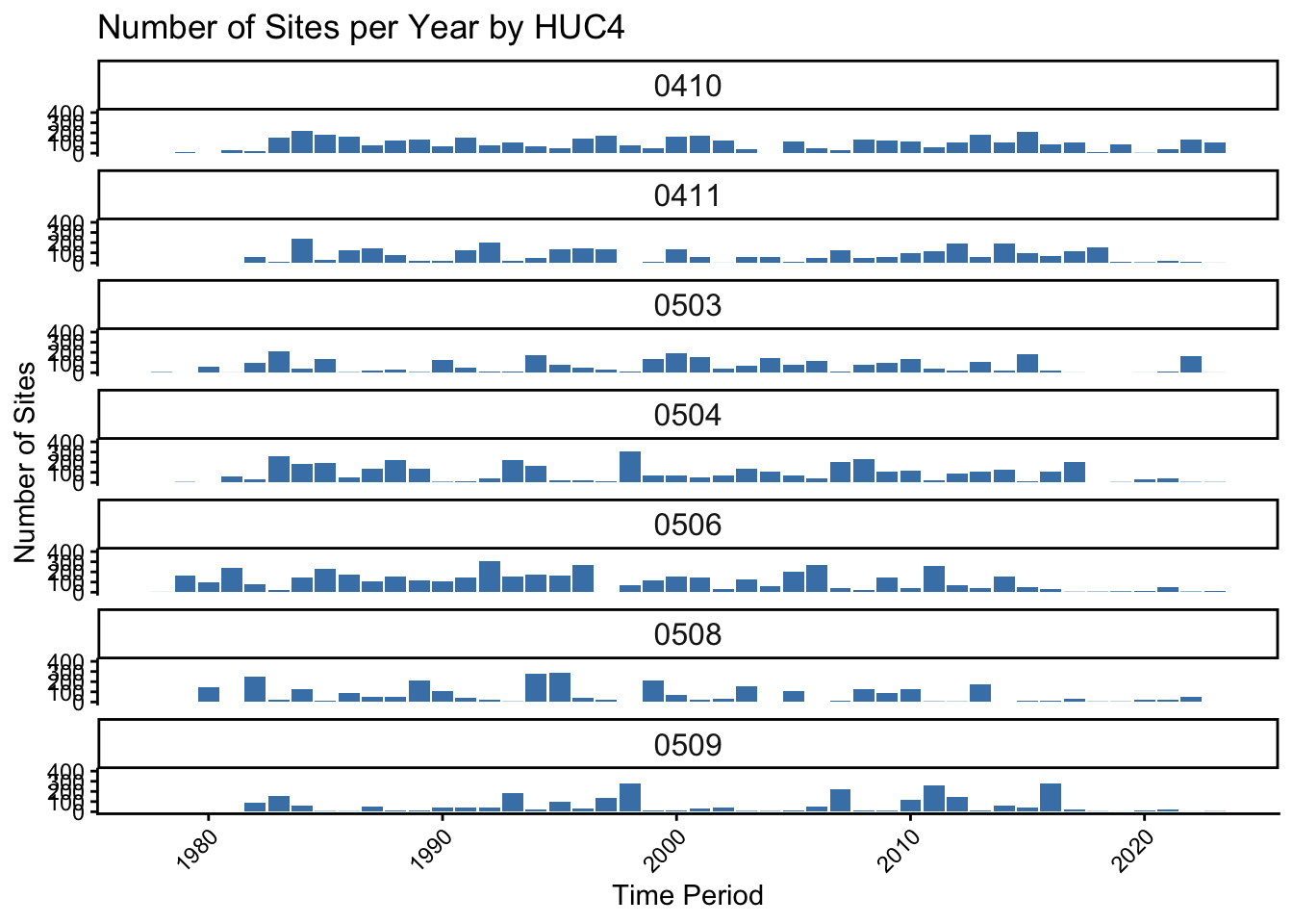
Moving on to bug data
dat2 <- bugs |> left_join(stations) |> left_join(bugcodes) |>
### separate out huc levels
mutate(
huc12 = huc,
huc8 = str_remove(huc, "-.*"),
huc6 = str_sub(huc8, 1, 6),
huc4 = str_sub(huc8, 1, 4)
) |>
### filter out under-represented hucs - based on CAP review
filter(!huc4 %in% c("0512", "0412", "")) |>
mutate(storesheet = paste(storet, sheet, sep = "_")) |>
### classify big and small rivers ---
mutate(river_class = case_when(
da > 500 ~ 'Large',
TRUE ~ 'Small')
)Joining with `by = join_by(latdd, longdd, storet, da)`
Joining with `by = join_by(taxa)`nacheck(dat2) station latdd longdd
0 0 0
watertype storet storeyr
0 0 0
sheet byear da
0 0 0
taxa taxaname quant
0 0 176593
qual pa name
0 0 0
station_id alife river
0 608 1477
alu cold basin
0 25114 0
rivercode rm dcode
0 0 0
huc station_type county
0 0 0
badflag refs eco
0 0 0
species_code species_name itis_taxon_id
0 0 0
family_code family_name reference_id
25346 25313 78803
species_group trophic_function is_tolerant
0 2757 0
pollution_tolerance is_sensitive is_coldwater
3473 0 0
ohio_endangered is_rare is_small_river_species
604491 0 0
is_large_river_species max_count last_updated_userid
0 606422 0
last_updated_date weighted_ici_score weighted_ici_count
0 1432 1432
wqx_name huc12 huc8
0 0 0
huc6 huc4 storesheet
0 0 0
river_class
0 Explore invertebrate survey effort
dat2 |>
group_by(huc4, byear) |>
summarize(
surveys = n_distinct(storesheet),
sites = n_distinct(storet),
.groups = 'drop'
) |>
ggplot(aes(x = byear, y = surveys)) +
geom_bar(stat = 'identity', fill = 'steelblue') +
facet_wrap( ~ huc4, ncol = 1, scales = "fixed") +
scale_y_continuous(limits = c(0, 400)) +
labs(title = "Number of Sites per Year by HUC4", x = "Time Period", y = "Number of Sites") +
theme_classic() +
theme(strip.text = element_text(size = 12),
axis.text.x = element_text(angle = 45, hjust = 1))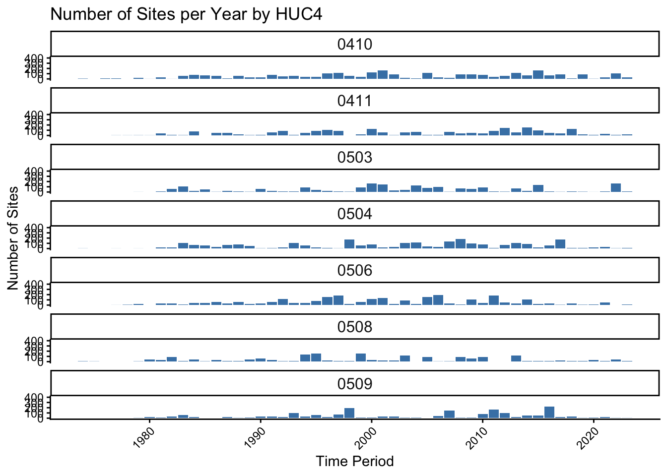
Clipping shapefiles in R
Example from Mack PhD Work
Below we showcase code that can be used to generate a clip a shapefile to the extent of another shapefile in R
Housekeeping
Load necessary packages
if you do not have librarian installed, you will need to install it first
#install.packages('librarian')
librarian::shelf(tidyverse, sf, mapview, ggspatial)Load necessary data
fl <- st_read('../../../R/shapefiles/fce_shapefiles/Florida_State_Boundary.shp')Reading layer `Florida_State_Boundary' from data source
`/Users/mack/Library/CloudStorage/Dropbox/R/shapefiles/fce_shapefiles/Florida_State_Boundary.shp'
using driver `ESRI Shapefile'
Simple feature collection with 1 feature and 4 fields
Geometry type: MULTIPOLYGON
Dimension: XY
Bounding box: xmin: -87.63493 ymin: 24.52104 xmax: -80.03132 ymax: 31.0002
Geodetic CRS: WGS 84Plot to check out the spatial file Here I use plot() with st_geometry() to take a quick look. The st_geometry() function removes the attributes from the spatial file so you see only see one file. See below
plot(fl)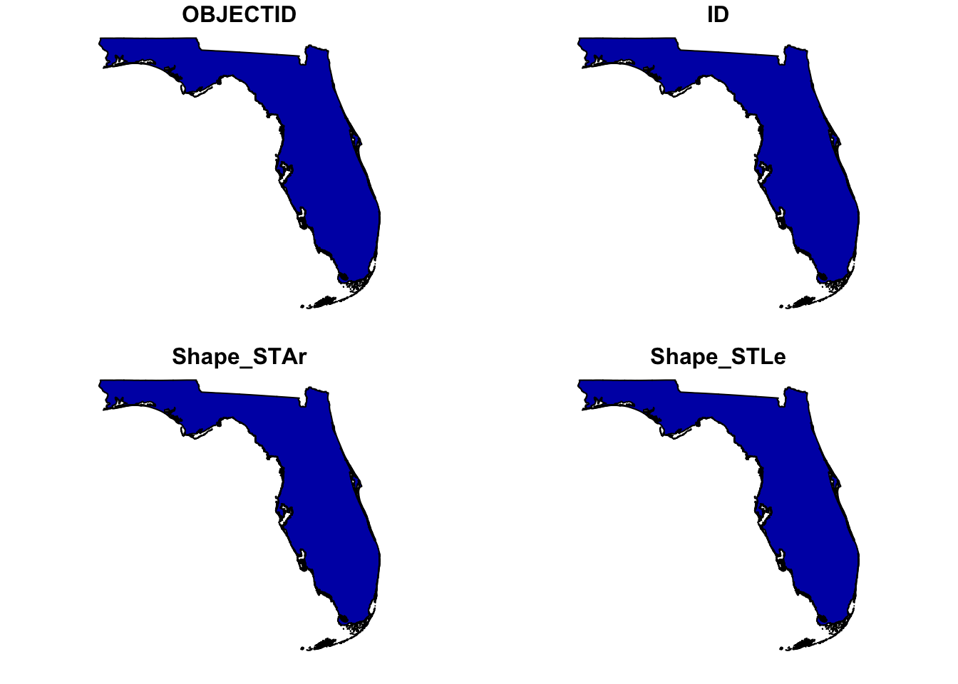
versus…
plot(st_geometry(fl))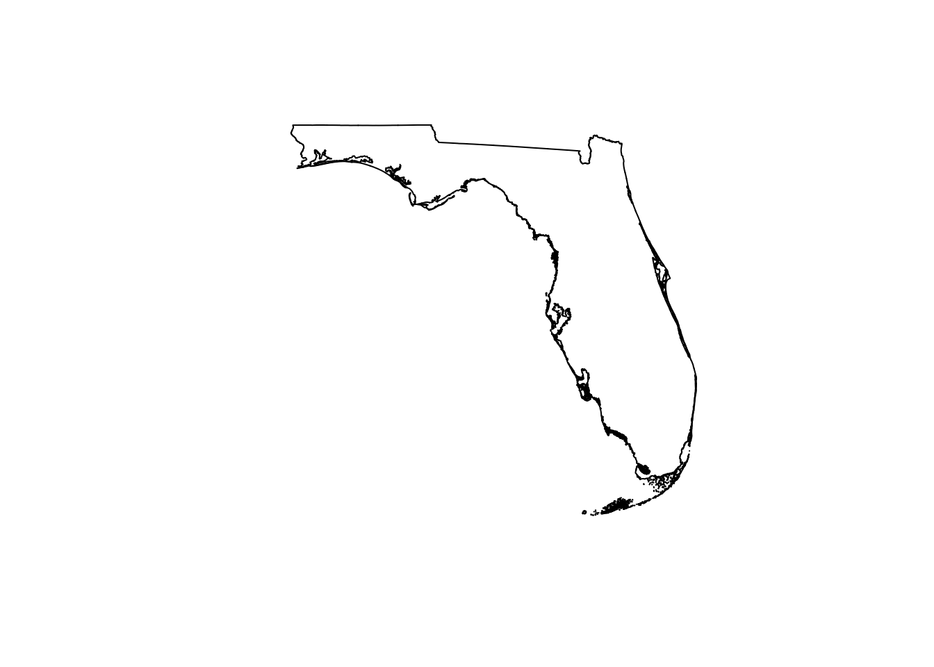
However, the mapview() is also really cool.. lets you pan in and out on your spatial file
mapview(fl)Load and reproject the shapefiles we put together in QGIS
Here, we load the and re-project the Shark River .shp file. We re-project this to UTM Zone 17N (EPSG:26917) which is representative of Southwest Florida
river <- st_read('../../../R/shapefiles/sharkriver-shapefiles/sharkriver_clean/SharkRiverClean.shp')Reading layer `SharkRiverClean' from data source
`/Users/mack/Library/CloudStorage/Dropbox/R/shapefiles/sharkriver-shapefiles/sharkriver_clean/SharkRiverClean.shp'
using driver `ESRI Shapefile'
Simple feature collection with 3 features and 2 fields
Geometry type: MULTIPOLYGON
Dimension: XYZ
Bounding box: xmin: 481890.7 ymin: 2798524 xmax: 514382.6 ymax: 2816786
z_range: zmin: 0 zmax: 0
Projected CRS: NAD83 / UTM zone 17Nriver <- st_transform(river, crs = 26917)
plot(st_geometry(river))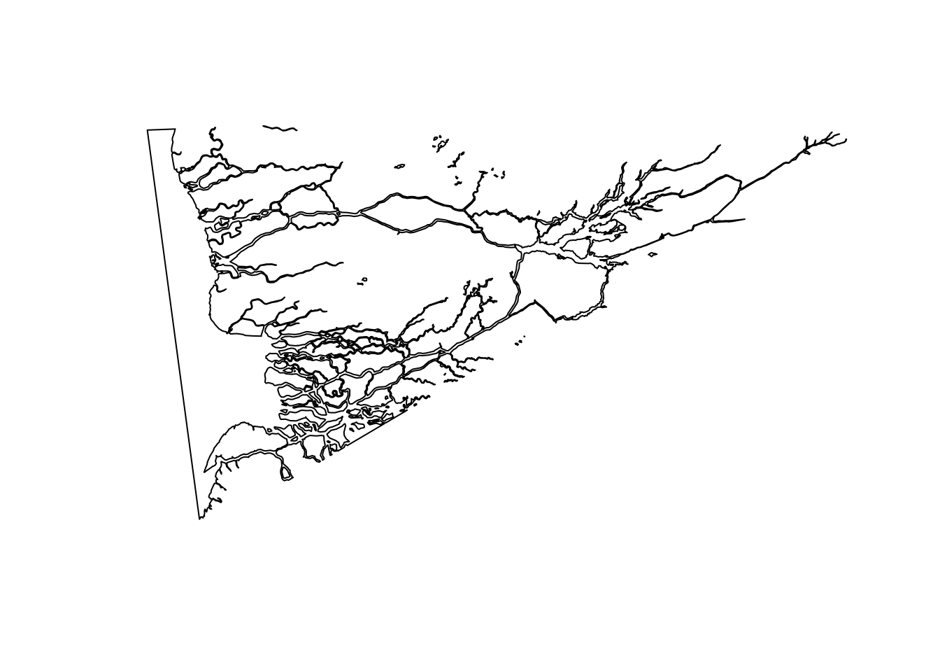
Do the same thing for our ‘river zones’
zones <- st_read('../../../R/shapefiles/sharkriver-shapefiles/zones_clean/SharkRiverZonesClean.shp')Reading layer `SharkRiverZonesClean' from data source
`/Users/mack/Library/CloudStorage/Dropbox/R/shapefiles/sharkriver-shapefiles/zones_clean/SharkRiverZonesClean.shp'
using driver `ESRI Shapefile'
Simple feature collection with 12 features and 1 field
Geometry type: POLYGON
Dimension: XY
Bounding box: xmin: -81.1562 ymin: 25.31597 xmax: -80.85419 ymax: 25.46635
Geodetic CRS: WGS 84zones <- st_transform(zones, crs = 26917)
plot(st_geometry(zones))
Clipping the Shark River shapefile to the River Zone shapefile
First, validate the geometry of each .shp using the st_make_valid(). This repairs any self-intersection, duplicate vertices, etc. that would otherwise result in failure of the clipping operation
river_valid <- st_make_valid(river)
zones_valid <- st_make_valid(zones) |> rename(Zone = geometry)Finally, clip the river to the zone shapefile so we don’t have sections of river showing outside of the zones in our map
river_clipped <- st_intersection(river_valid, zones_valid)Warning: attribute variables are assumed to be spatially constant throughout
all geometriesFor fun, create an inset of the state of Florida
inset <- ggplot() +
# adding in the state of FL
geom_sf(data = fl, fill = 'grey', color = 'black') +
# create rectangle to separate from larger map
geom_rect(aes(xmin = -81.252753, xmax = -80.749544,
ymin = 25.266087, ymax = 25.576524),
color = 'black', fill = NA, linewidth = 1) +
# place the name of the state we are looking at in the GOM
annotate("text", x = -85.34, y = 24.97, label = "Florida, USA",
fontface = "bold", size = 5) +
theme_bw() +
theme(
axis.title = element_blank(),
axis.text = element_blank(),
axis.ticks = element_blank(),
axis.ticks.length = unit(0, "pt"),
panel.grid.major = element_blank(),
panel.grid.minor = element_blank(),
# make the ocean blue :)
panel.background = element_rect(fill = 'aliceblue', color = NA),
panel.border = element_rect(fill = NA, color = 'black', linewidth = 2),
# limits margins so it fits nicely in the larger map
plot.margin = grid::unit(c(0, 0, 0, 0), "null"),
legend.position = 'none'
)
inset 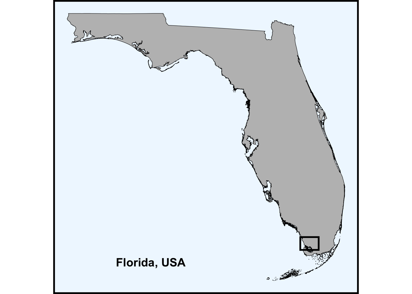
Create a label df for the different parts of the map. I spent a lot of time (too much to admit) trying to line these up. I am sure there is a better way to do it, but this does work :)
labels <- data.frame(
name = c("Tarpon Bay", "Gulf of \nMexico", "Rookery Branch",
"Otter Creek"),
lon = c(-80.972, -81.145, -80.866, -80.940),
lat = c(25.424, 25.3592, 25.445, 25.459)
) |>
st_as_sf(coords = c("lon", "lat"), crs = 4326) |>
st_transform(crs = 26917)Check out your awesome map with clipped river
ggplot() +
# lay the map of FL down
geom_sf(data = fl, fill = 'grey', color = NA) +
# lay the river down
geom_sf(data = river_clipped, fill = 'aliceblue', color = NA) +
# lay your zones down
geom_sf(data = zones_valid, fill = NA, alpha = 0.2,
aes(color = 'Zone'), linewidth = 1) +
# place your labels in the map
geom_sf_text(data = labels, aes(label = name), size = 4, fontface = "italic") +
# add in your scale bar
annotation_scale(location = "br", width_hint = 0.3,
bar_cols = c("black", "aliceblue"), text_cex = 1.0) +
# add in your north arrow
annotation_north_arrow(location = "tl", which_north = "true",
style = north_arrow_fancy_orienteering(
fill = c("black", "aliceblue"),
line_col = "black"),
height = unit(2.0, "cm"), width = unit(2.0, "cm")) +
# zoom to Shark River extent lat/lon limits
coord_sf(xlim = c(-81.15, -80.855), ylim = c(25.32, 25.465)) +
# manually assign colors for points/lines on the map - just zones here
scale_color_manual(values = c("Zone" = "black")) +
theme_bw() +
# Embed the inset map as a grob - stands for graphical object
annotation_custom(
ggplotGrob(inset),
xmin = -80.935217, xmax = -80.843471,
ymin = 25.317539, ymax = 25.415402) +
theme(
axis.title = element_blank(),
axis.text = element_blank(),
axis.ticks = element_blank(),
panel.grid = element_blank(),
panel.background = element_rect(fill = "aliceblue"), # ocean fill
plot.title = element_text(size = 18, hjust = 0.5),
legend.title = element_blank(),
legend.background = element_rect(fill = 'aliceblue'),
legend.position = c(0.928, 0.695), # normalized (0–1) position within panel
legend.box.background = element_rect(fill = NA, color = 'black', linewidth = 2),
legend.text = element_text(size = 12, face = 'bold')
)Warning in st_point_on_surface.sfc(sf::st_zm(x)): st_point_on_surface may not
give correct results for longitude/latitude data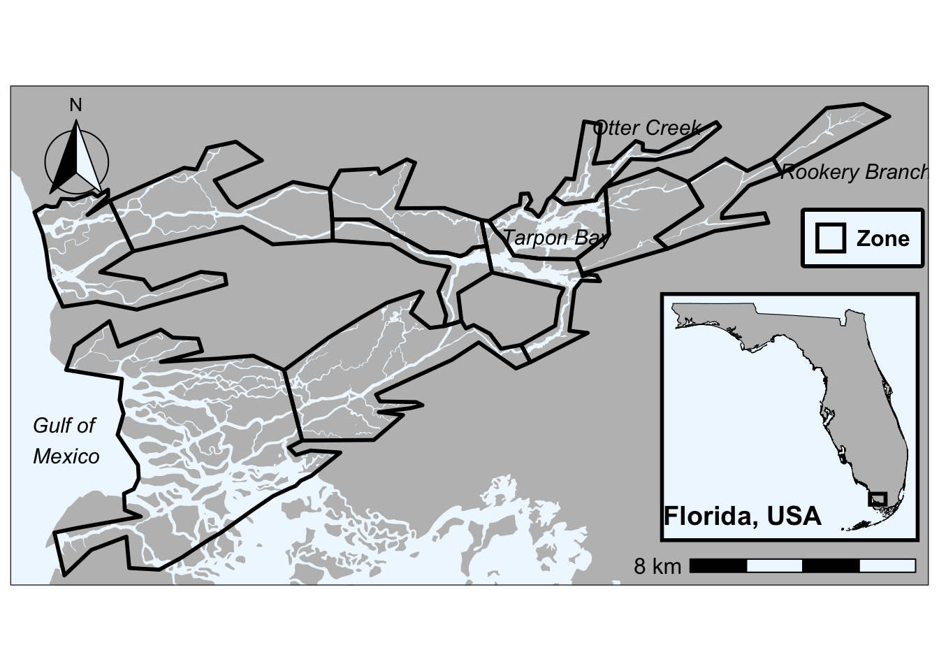
Check out what the river shapefile would look like if it wasn’t clipped
ggplot() +
# lay the map of FL down
geom_sf(data = fl, fill = 'grey', color = NA) +
# lay the river down
geom_sf(data = river_valid, fill = 'aliceblue', color = NA) +
# lay your zones down
geom_sf(data = zones_valid, fill = NA, alpha = 0.2,
aes(color = 'Zone'), linewidth = 1) +
# place your labels in the map
geom_sf_text(data = labels, aes(label = name), size = 4, fontface = "italic") +
# add in your scale bar
annotation_scale(location = "br", width_hint = 0.3,
bar_cols = c("black", "aliceblue"), text_cex = 1.0) +
# add in your north arrow
annotation_north_arrow(location = "tl", which_north = "true",
style = north_arrow_fancy_orienteering(
fill = c("black", "aliceblue"),
line_col = "black"),
height = unit(2.0, "cm"), width = unit(2.0, "cm")) +
# zoom to Shark River extent lat/lon limits
coord_sf(xlim = c(-81.15, -80.855), ylim = c(25.32, 25.465)) +
# manually assign colors for points/lines on the map - just zones here
scale_color_manual(values = c("Zone" = "black")) +
theme_bw() +
# Embed the inset map as a grob - stands for graphical object
annotation_custom(
ggplotGrob(inset),
xmin = -80.935217, xmax = -80.843471,
ymin = 25.317539, ymax = 25.415402) +
theme(
axis.title = element_blank(),
axis.text = element_blank(),
axis.ticks = element_blank(),
panel.grid = element_blank(),
panel.background = element_rect(fill = "aliceblue"), # ocean fill
plot.title = element_text(size = 18, hjust = 0.5),
legend.title = element_blank(),
legend.background = element_rect(fill = 'aliceblue'),
legend.position = c(0.928, 0.695), # normalized (0–1) position within panel
legend.box.background = element_rect(fill = NA, color = 'black', linewidth = 2),
legend.text = element_text(size = 12, face = 'bold')
)Warning in st_point_on_surface.sfc(sf::st_zm(x)): st_point_on_surface may not
give correct results for longitude/latitude data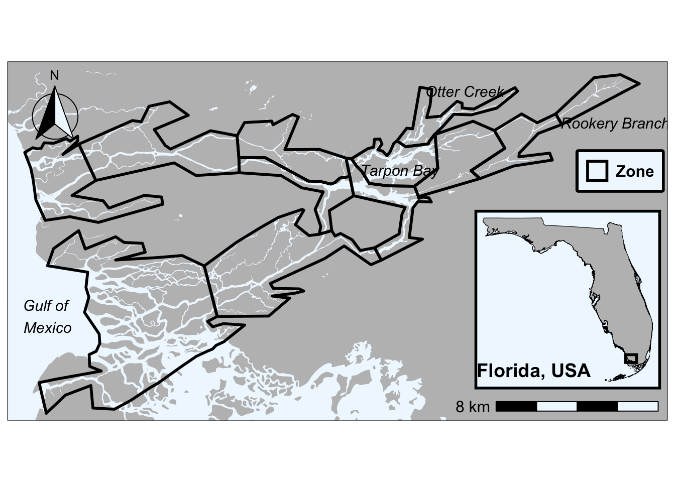
Hierarchical Partitioning
Example from preliminary analyses of mussel life history data
Below we showcase code that can be used to partition independent effects of predictor metrics nested within each group of predictors used in variance partitioning analyses :)
Housekeeping
Load necessary packages
if you do not have librarian installed, you will need to install it first
#install.packages('librarian')
librarian::shelf(
tidyverse, ggplot2, skimr, patchwork, cowplot, tibble, vegan, rdacca.hp, eulerr, corrplot, grid
)First, need to run base function rdacc.hp() - see here to learn more about the package and why it was authored in the first place
hp_res <- rdacca.hp(
# distance matrix (same one from dbRDA goes here)
dist_mat,
# predictors from each of the forward-selected models go here
pred_mat[, c("magnitude", "developed", "pasture_hay", "watershed_area")]
)Next, we generate a dataframe that we can visualize the data from using the ggplot package. First we are extracting the results (i.e., hp_res$Hier.part)
hp_df <- hp_res$Hier.part |>
as.data.frame() |>
# convert row names to column (new column is variable) for plotting
rownames_to_column("variable") |>
mutate(
# create the label for each predictor
# here I am rounding the % independent effect and adding a "%" for clarity
label = paste0(round(`I.perc(%)`, 1), "%"),
# assign colors - whatever we want, but should be consistent
color = case_when(
# hydrology
variable %in% c("magnitude") ~ "#4E7D96",
# land use
variable %in% c("developed", "pasture_hay") ~ "#A47551",
# connectivity
variable %in% c("watershed_area") ~ "#4A7C59"
)
)Plot it out :)
hp_df |>
# ordering the variables so they cascade down (relies on coordflip)
mutate(variable = factor(variable, levels = variable[order(`I.perc(%)`)])) |>
ggplot(aes(x = variable, y = `I.perc(%)`, fill = color)) +
geom_col(width = 0.6, color = "white", alpha = 0.6) +
geom_text(aes(label = label), hjust = -0.2, fontface = "bold", size = 4) +
scale_fill_identity() +
#renaming predictor variables for clarity
scale_x_discrete(labels = c(
"magnitude" = "Flow\nmagnitude",
"developed" = "Developed\n(% cover)",
"pasture_hay" = "Pasture/hay\n(% cover)",
"watershed_area" = "Watershed\narea"
)) +
scale_y_continuous(
# can play with this - could probably do 0,40 for most
limits = c(0, 50),
expand = c(0, 0),
name = "Independent effects (%)"
) +
labs(x = NULL) +
# flips plot on side - looks better IMO
coord_flip() +
# remove grid lines
theme_classic() +
# typical theme I use for most of my figs but can be tweaked
theme(
strip.text = element_text(size = 16, face = "bold", colour = "black"),
strip.background = element_blank(),
axis.text.x = element_text(size = 12, face = "bold", color = "black"),
axis.text.y = element_text(size = 12, face = "bold", color = "black", hjust = 0.5),
axis.title = element_text(size = 14, face = "bold", color = "black"),
plot.title = element_text(size = 16, face = "bold", color = "black", hjust = 0.5),
panel.grid.major = element_blank(),
panel.grid.minor = element_blank(),
panel.border = element_blank(),
panel.background = element_blank(),
axis.line = element_line(color = "black"),
legend.position = "right",
legend.text = element_text(size = 7, face = "bold", color = "black"),
legend.background = element_blank(),
legend.title = element_text(size = 10, face = "bold", color = "black", hjust = 0.5)
)